

Voronoi Tessellation#
The full implementation of the GCVT is available on the DSG-Applications repository.
This example demonstrates how to perform Geodesic Centroidal Voronoi Tessellation (GCVT) on 3D meshes using the Mesh-LBFGS second-order optimiser provided by this library.
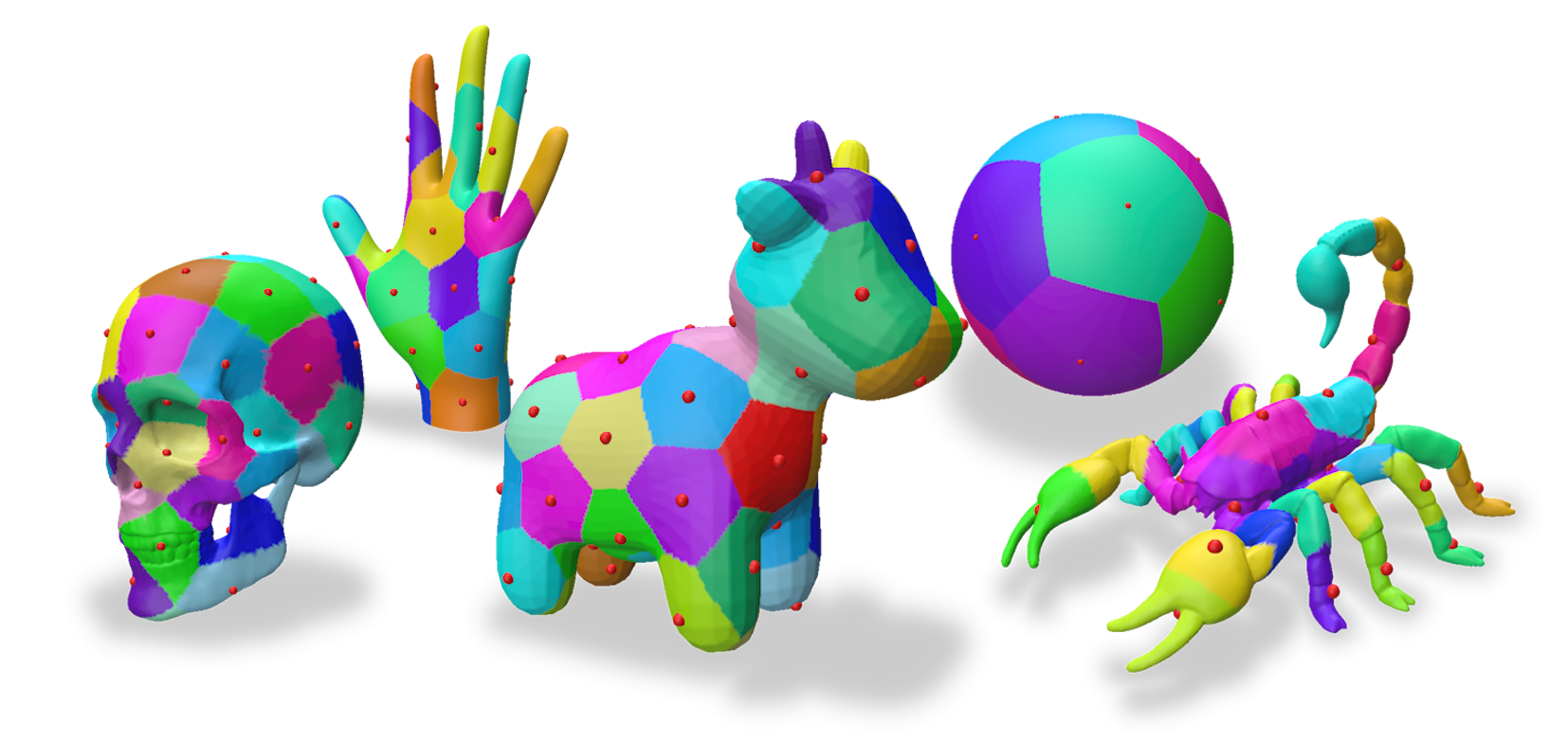
GCVT examples using the Mesh-LBFGS optimiser.#
GCVT aims to partition a manifold \(\mathcal{M}\) into \(S\) regions \(\{\Omega_i\}_{i=1}^S\) based on the distance to a set of seeds \(\mathcal{S} = \{s_i\}_{i=1}^S \in \mathcal{M}\). A tessellation is centroidal when each seed \(s_i\) coincides with the Karcher mean (center of mass) of its respective Voronoi cell \(\Omega_i\).
Our implementation leverages Mesh-LBFGS, the second-order Riemannian optimiser designed specifically for 3D meshes, which utilizes our parallelized GPU exponential map and parallel transport operators.
Mathematical Formulation#
To find the optimal seed positions, we minimize the following loss function:
Where:
\(A(x)\): The vertex area, defined as one-third of the sum of areas of triangles connected to vertex \(x\).
\(\rho(x)\): A density function defined via the scalar heat kernel.
\(Log_{s_i}(x)\): The Riemannian logarithm map finding the shortest vector from seed \(s_i\) to vertex \(x\).
In practice, we compute the Log map at each seed, and compute a Karcher mean for each Voronoi cell using the Vector Heat Solver provided by the Potpourri3D library. This Karcher mean gives us the direction in which to move each seed, which gives us the gradient of the loss function with respect to the seed positions. We can then use Mesh-LBFGS to optimize the seed positions iteratively until convergence.
Optimization via Mesh-LBFGS#
We first define the loss function used for optimization, which computes the energy and its gradient with respect to the seed positions.
from digeo.optim import MeshLossFunc
from digeo import Mesh, MeshPointBatch
import potpourri3d as pp3d

class LossGCVT(MeshLossFunc):
    def __init__(self, mesh: Mesh):
        super().__init__()
        self.solver = pp3d.MeshVectorHeatSolver(
            mesh.positions.detach().cpu().numpy(),
            mesh.triangles.detach().cpu().numpy(),
            t_coef=0.25,
        )
        self.regions = None

    def compute(self, mesh: Mesh, x: MeshPointBatch):
        grad, regions, loss = get_karcher_mean(self.solver, mesh, x)
        self.regions = regions
        return loss, grad

    def get_logs(self):
        return {"regions": self.regions}
Once the loss function is defined, we can initialize the seed positions and run the optimization loop using Mesh-LBFGS.
from digeo import load_mesh_from_file
from digeo.ops import uniform_sampling
from digeo.optim import mesh_lbfgs

mesh = load_mesh_from_file("path/to/mesh.obj")
initial_seeds = uniform_sampling(mesh, num_samples=50)
loss_func = LossGCVT(mesh)

seeds, logs = mesh_lbfgs(mesh, initial_seeds, loss_func)